Here be Dragons: Gaps in the human genome

Know thyself

The Human Genome Project formally began in 1990 and was declared complete in April 2003. After thirteen years and billions of dollars, researchers produced a sequence of more than 3 billion nucleotides. The sequential string of A, C, G, and T was the most accurate and specific representation of our own genetic code that had ever been produced.

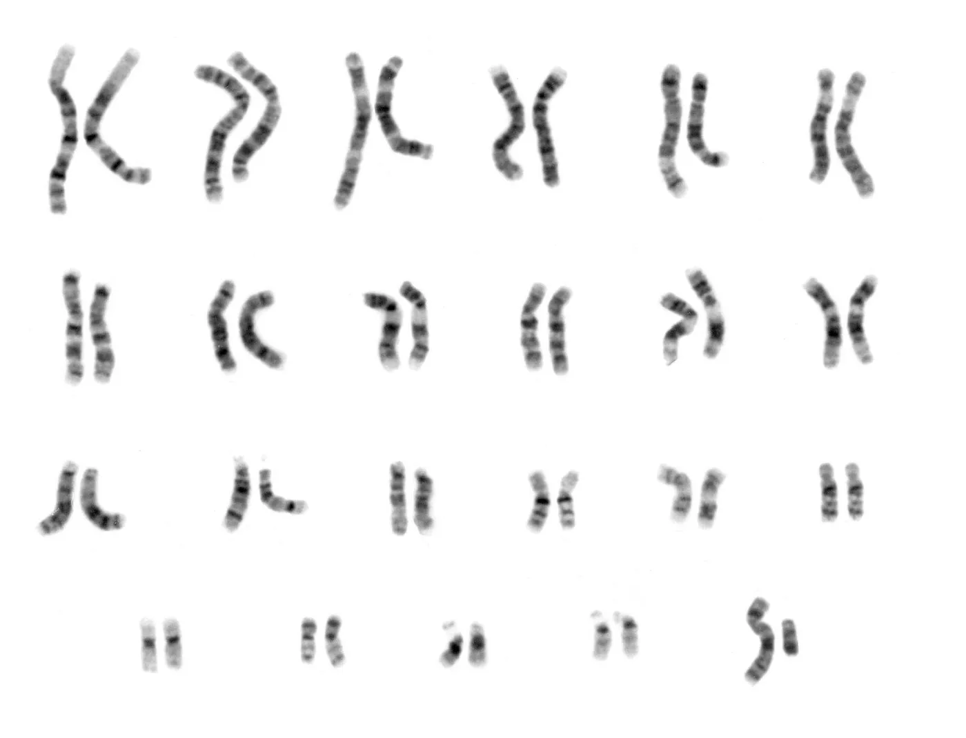
Just as human explorers made the first maps of the world in order to more easily navigate it, genetic explorers made the first map of our genome. Incomplete as it was, we had finally committed the consensus sequence of our internal genetic code to the digital record. Prior research went back more than a hundred years and had already established the principals of genetic inheritance, found that genetic information is carried by nucleic acids, and had discerned the structure of the DNA molecule. Before it had been sequenced, our map of genetic knowledge amounted to little more than a rough sketch of coastlines of the major continents. The precise location and function of genes encoded in the banded information carrying molecules was still unknown, and subject to myth and speculation. Here be dragons.

The “complete” 2003 human genetic reference sequence was, in fact, far from complete. It was composed of DNA samples from several individuals distilled down to a string of bases covering about 92% of the entire genome. Most of the work concentrated on the transcriptionally active euchromatic regions that encode the ~20,000 known protein producing genes and gene regulating sequences. The highly repetitive heterochromatic regions (including centromeres and telomeres) were not included in the initial release. This was largely due to the difficulty of accurately sequencing them, as well the suspicion that these regions were largely useless accretions of “junk DNA”.

In September 2020, the first full telomere-to-telomere (T2T) sequence was produced for every human chromosome (except Y). Instead of using a single human or a composite of several individuals, the genetic material came from a complete hydatidiform mole (CHM). A CHM is the result of a complication of human pregnancy that occurs when an ovum with no nucleus is present. The egg would ordinarily be rejected by the uterus, but in rare cases it can be fertilized by one or more sperm. When fertilized with a single sperm (which, like a healthy ovum, is haploid) its genome replicates itself to provide the required second copy. The result is a non-viable diploid cell with nearly identical sets of chromosomes.

Using haploid DNA significantly reduced the complexity of sequencing. By using a combination of long read and short read sequencing technologies, an extremely high quality single haplotype was produced. Nearly all of the highly complex and repetitive gaps remaining in the genetic reference have been traversed, and T2T has finally filled in the dark edges and deep jungles of the map. Our understanding of the complete structure of our chromosomes has never been more clear.

And yet, the dragons still haunt us.

A map is not the territory it represents, but, if correct, it has a similar structure to the territory, which accounts for its usefulness.
– Alfred Korzybski, Science and Sanity, 1933

Sequencing technology has improved significantly since 2003, and several revisions to the human reference have been produced. But as more genomes from humans with diverse geographic backgrounds become available for research, it has become apparent that the standard reference is “too European”.

While human sequences differ from each other by 0.1% to 0.4%, that still accounts for millions of differences with respect to the reference. As the genetic diversity of a DNA sample diverges from reference, the number of variants increases.

The human reference’s 3.2 billion nucleotides obviously cannot reflect the genetic diversity of every human on the planet. But as long as we remember that it is only an approximation of the genomes that went into its construction, it can be useful as a point of departure.

Short roads, long roads

A DNA “read” is a single uninterrupted sequence of bases produced by a sequencer. Short read sequencing (also called Next Generation Sequencing or NGS) produces reads about 100 to 300 bases long, at a base error rate of about 0.1%. Approximately one in one thousand bases is expected to have an error, which is typically corrected for by oversampling the genome 30 to 50x. Illumina is the dominant provider of sequencers for NGS.

Long read sequencing (also called third-generation sequencing) can produce reads that span hundreds of kilobases to multiple megabases, at a base error rate of about 1%. Approximately one in one hundred bases is expected to have an error, and typical oversampling for whole genome applications is 5 to 10x. PacBio and Oxford Nanopore are the largest providers of long read sequencing technology.

Long reads are significantly easier to assemble than short reads, and can traverse regions that are otherwise difficult to resolve. This February 2020 article in Genome Biology provides a thorough comparison of the advantages and disadvantages of long read vs. short read sequencing.

While the results of the telomere-to-telomere project are impressive, it was a significant undertaking. It took researchers a year and more than $50,000 to produce the full sequence. They ultimately used a combination of long reads and short reads to make the final assembly.

This time and cost per genome for that level of detail is obviously not (yet) scalable. When people talk about the $1000 genome, they are referring to short read (NGS) whole human genome sequencing experiments. Short reads can be produced by the sequencer in parallel, resulting in much higher volume and much lower costs compared to long read sequencing.

Taking the shortcut

Whole genome sequencing for a single human sample can be accomplished in about one day using NGS sequencers. After the DNA extraction and preparation has been performed and the material is run through the sequencer, reads are provided in FASTQ format. This includes the base sequence, the read’s mate pair, and the sequencer’s best guess at the quality of the call for each base. A quality control check is typically performed at this stage to filter out reads containing too many low quality bases or that otherwise look like outliers.

No other information about a read’s original location in the genome is available at this stage. The reads must first be assembled back into a meaningful order using only the short nucleotide sequence present in the read.

While de novo human assembly is possible, it is much more feasible and generally less error-prone to attempt to place reads by mapping them to the genetic reference. Mapping aligners like BWA are very efficient at finding the best location for each read that at least partially matches the reference. Hardware accelerated products can do the job even faster.

But even with high-coverage sequencing runs, variations in read coverage happen for a number of reasons. PCR amplification underrepresents GC rich regions, and even PCR-free analysis reduces, but does not eliminate, GC bias. Mappers can only work with the reads as provided by the sequencer, and errors in the source material tend to be amplified in the final analysis. Consistently incorrect base calls can lead to mapping errors. Incorrectly mapped reads may artificially increase or decrease relative coverage, leading to spurious variant calls. Homozygous variants in areas of low coverage may be incorrectly called as heterozygous, or may not be called at all.

🐲 Dragon #1: sequencing bias. The sequencing platform itself is never completely free of bias, and may introduce detectable systematic errors that lead to incorrect variant calls.

When as many reads as possible have been placed on the reference, the result is a pile-up of overlapping reads sorted by chromosome and position. Any reads that do not match reference or otherwise support the assembly are typically ignored or filtered out entirely. The remaining reads are then typically saved in BAM or CRAM format, and genetic variants are called against the reference using callers such as GATK or Sentieon.

Miles still to go

Mapping reads to reference is not a trivial task.

Since a read may have come from either DNA strand, it may have been sequenced in the 5’ to 3’ (forward) direction or 3’ to 5’ (reverse). But the genetic reference only consists of a single string of bases all read in the forward direction. Reads sequenced in the reverse direction therefore must be reversed and complementary DNA bases substituted in order to match reference. The reads encoded in FASTQ do not (and prior to mapping and alignment, cannot) indicate which reads require reverse complementing.

Then there’s the matter of those “unmappable” reads. The more a sample diverges from the reference, the more likely any given read will not be able to be placed by the mapper. Surely those reads can’t all be errors, but if they can’t be placed in an assembly they can’t be used.

And so we stumble upon another dragon in the map.

🐲 Dragon #2: reference bias. Your choice of genetic reference directly dictates the number and quality of your variant calls.

This 2017 article in Genome Research titled “Genome graphs and the evolution of genome inference” concisely summarizes the reference bias problem:

Reference allele bias is the tendency to underreport data whose underlying DNA does not match a reference allele. […] In order to map correctly, reads must derive from genomic sequence that is both represented in the reference and similar enough to the reference sequence to be identified as the same genomic element. When these conditions are not met, mapping errors introduce a systematic blindness to the true sequence.

Clearly the choice of reference is an important decision when mapping reads. It is critical to choose a genetic reference that matches your cohort as closely as possible. But how can you choose the best map for the journey if the cartographers are still at work?

Fork in the road

Until 2021, there were two major revisions to the reference in common use: GRCh37 (hg19) and GRCh38 (hg38). With the completion of the telomere-to-telomere project, CHM13 is likely to become a popular choice going forward. A number of other variations of these sequences are also in common use.

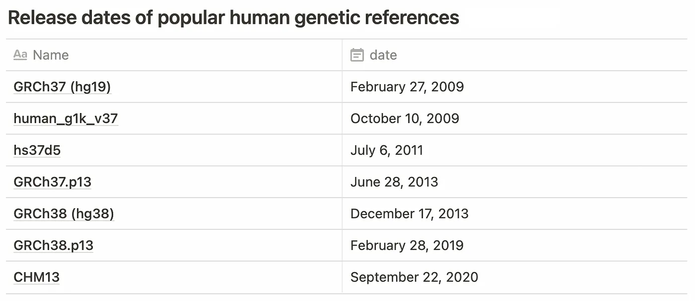
Aside from vintage, there is the question of “flavor”. Several variations exist for each reference to account for differences in chromosome naming convention (eg. 1 vs. chr1 vs. CM000663.2), the addition of alternate assemblies, and the inclusion of decoy sequences to assist with mapping common sequences that don’t appear on the standard reference (such as EBV).

If you find the options a bit dizzying, you are not alone. Heng Li has an excellent blog post about reasons why you might choose one over another. An entire module of BioGraph is devoted to simplifying the process of handling multiple references.

Practically speaking, vast numbers of genomes have already been mapped to some reference. If you want to use that data and the genomes were not mapped to the reference that you have chosen for the rest of your analysis, you have some work ahead of you. You will need to spend the compute time to remap your reads to the new reference, produce a new BAM, and call variants against it. This is also true of variant annotation databases like dbSNP and ClinVar: if your variant calls use a different reference, you are out of luck.

🐲 Dragon #3: reference lock-in. There are many references, all with different attributes and revisions, and changing references is computationally expensive.

Even if you control the genome analysis pipeline for your organization, times change. Your scientists will eventually want to use a new reference in order to reduce reference bias and produce better quality variant calls.

Is there an objectively “best” reference? Of course not. Your choice of reference depends on your source genomes and your analysis goals. But if your pipeline includes structural variation calling, the choices are particularly bleak. This quote is also from Genome graphs and the evolution of genome inference, regarding reference bias:

In the context of genetic variant detection, this problem is most acute for structural variation. Entirely different classes of algorithm are required to discover larger structural variation simply because these alleles are not part of the reference. Furthermore, the numerous large subsequences entirely missing from the reference in turn surely contain population variation. Describing these variants and their relationships is simply not possible with the current reference model.

Unfortunately, reference bias can hinder the utility of using short read sequencing for the detection of structural variations.

🐲 Dragon #4: poor representation of structural variations. Mapping aligners can only map reads to recognized sequences, reducing sensitivity for large SVs that span multiple read lengths.

Have we outgrown the usefulness of simple maps? Some researchers believe so. It is possible that a better human reference could be built by using a data structure that is more analogous to our genetic diversity: the graph.

A map of all maps: graph references

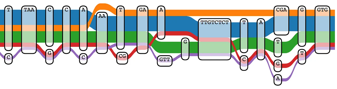
The limitations of the linear reference have been known for some time. This 2017 paper titled “Genome Graphs” examines the technical advantages to a graph approach in detail. Instead of a single linear haplotype for each chromosome, a graph structure can include multiple alleles derived from several representative human samples. Using a graph reference can reduce the number of spurious variant calls due to mapping errors, and more accurately reflect variants found in a specific subpopulation.

Producing a graph reference for a specific population (or including as much genetic diversity as possible to produce a pangenome) is not a small effort, and a number of projects are currently underway. The Human Genome Reference Program effort at the NIH is one such effort. A working group at the GA4GH has been developing pangenome tools and structures since 2014. The Human Pangenome Reference Consortium has recently produced data for 30 genomes from diverse genetic backgrounds using a variety of sequencing technologies. If you have access to high quality human assemblies and are feeling adventurous, you can even build your own graph reference using tools like minigraph or NovoGraph.

The graph is poised to replace the map as the preferred data structure representing human genetics. But it will clearly take some time for high quality genome assemblies to become available, standards to be released, and for analysis tools and variant databases to be able to take full advantage them.

Until then, the linear reference will continue to be our best tool for orienteering the genome.

But are we really making the best possible use of the maps we already have?

BioGraph: map the reference, graph the reads

After five years of development at Spiral Genetics, BioGraph is now free for academic use with full access to the source code.

👉 This brief overview only highlights some of the differences between BioGraph and traditional reference-based analysis. For a deeper dive into to the BioGraph technology, see our whitepaper.

BioGraph addresses many of the shortcomings of mapping to a linear reference by using novel methods. In contrast with BAM or CRAM (which maps reads to reference and sorts them by position), the BioGraph format stores reads in a highly compressed graph data structure sorted by sequence.

An arbitrary k-mer can be found in the graph in O(1) time for each base in the k-mer, regardless of the number of reads present. This enables novel sequenced-based discovery and genotyping methods that overcome the limitations of pure mapping based approaches. Since k-mer lookups are nearly free, detection and correction of sequencing bias is trivial, and limiting mapping operations reduces reference bias.

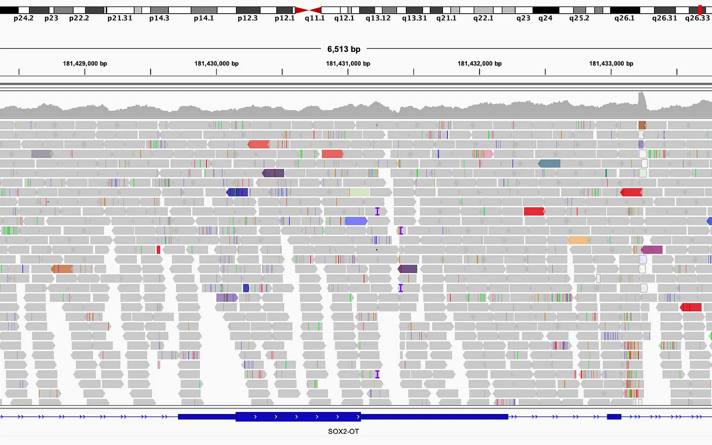
Remember those “unmappable” reads? BioGraph can assemble them to each other, enabling discovery of arbitrarily large insertions with full base resolution.

The BioGraph format itself is inherently reference-free. Variant discovery can be performed against the BioGraph using any desired reference without the need to remap the reads, thus avoiding reference lock-in.

BioGraph also creates a variant graph when genotyping across populations. A dynamic graph reference is built from the variant calls being genotyped. Any number of variants may be genotyped simultaneously, including variants found in other samples in a cohort. The “squaring off” pipeline improves variant recovery and genotyping at a far smaller computational cost compared to traditional methods by avoiding the need to remap the reads from every sample to reference.

Where to next?

The ideal genomic analysis of the future will perfectly describe the sequence of both alleles of every chromosome, from telomere to telomere. It will report a functional description of changes to known genes that could result in an alteration of expected protein expression, as well as structural abnormalities that might result in functional change. The function of newly discovered sequences will be predicted by sophisticated models. Large structural variants will be reported as a gain, loss, or change in function of impacted genes and gene regulation sequences with base level accuracy, even in complex and highly repetitive regions.

In 2021 it is technically possible but extremely time consuming and costly to produce such an analysis, even for a single individual. Tools like BioGraph help to maximize the utility of inexpensive short read analysis beyond discovering SNPs and small indels in coding regions.

Our understanding of human biochemistry may never be truly complete. But every new human sequenced means that another example of a working genetic system has been added to our collective knowledge. By reducing the cost and complexity of whole genome sequencing and extracting the maximum useful information from sequencing experiments, we have some hope of banishing those dragons and collectively finding new exciting paths to explore.